The three faces of diffusion models

Written by Zhicheng Jiang & Hanhong Zhao

Introduction

Diffusion models are a powerful class of generative models capable of producing high-quality samples from complex data distributions. The mathematical formulation of diffusion models is often quite complicated, either explaining in discrete Markov chains or continuous stochastic differential equations. However, in this post, we will try to explain the what the models are learning in a more intuitive way and reveal the three different faces of the diffusion models.

Mathematical Formulation

Before delving into the interesting parts, some math may be useful for illustrating the settings. So, let us start by reviewing the mathematical formulation of diffusion models. For these models, there is a hand-crafted forward/noising process, where the data is iteratively perturbed with noise and eventually approximates a standard normal distribution. On the other hand, they also have a learned reverse/denoising process, which aims to match the conditional probability distribution at each step.

Forward Process

Let us start with the forward process. More formally, the forward process can be expressed as:

\[p(x_t\mid x_{t-1}) = \mathcal{N}(x_t; \hat{\mu}_t(x_{t-1}), \hat{\sigma}_t(x_{t-1})^2\mathbf{I}),\qquad t=1,2,\ldots,T,\]

where $\hat{\mu}_t, \hat{\sigma}_t$ are simple functions (for example, in DDPM we have $\hat{\mu}_t(x)=\sqrt{1-\beta_t}x,\hat{\sigma}_t(x)=\sqrt{\beta_t}$, whereas $\beta_t$ are some hyperparameters, called the “diffusion schedule”).

The process starts with $x_0 \sim p_{\text{data}}$, and with properly selected $\beta_t$’s, we can ensure that $x_T \approx \mathcal{N}(0, I)$. We can further illustrate this in the figure below.

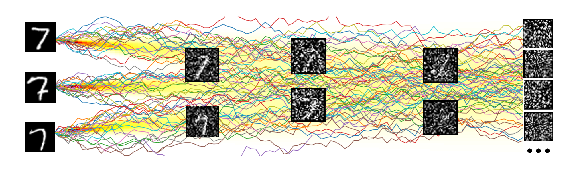
We can see that by adding a relatively small amount of noise at each step (denoted as a straight segment in each of the paths in the figure), the data distribution gradually transforms into the standard normal distribution.

Reverse Process

Now, let us focus on the reverse process, where the learning actually happens. As we have mentioned, the neural net is going to model the one-step “reversed” conditional distribution

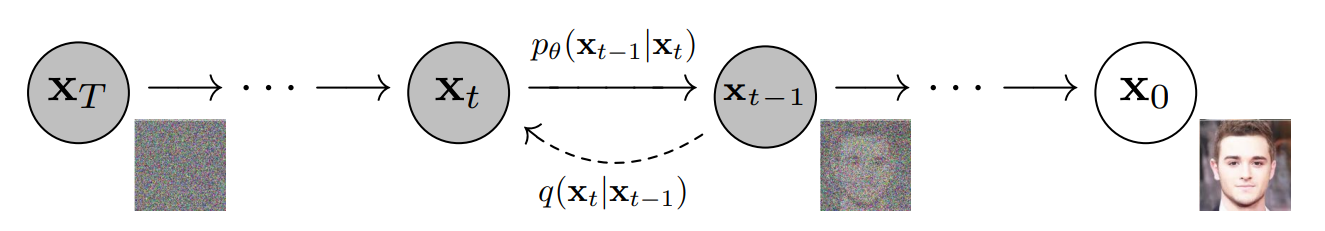
\[p_\theta (x_{t-1}\mid x_t)\approx p(x_{t-1}\mid x_t),\]

which is the essence of the reverse process: as long as this is modeled correctly, we can then sample a Gaussian noise from $p(x_T)=\mathcal{N}(0,1)$, and then iteratively sample $x_{t-1}\sim p_\theta(x_{t-1}\mid x_t)$ to get a sample $x_0$, which matches the original data distribution $p_{\text{data}}(x_0)$ (or to make notations simpler, just $p(x_0)$).

This can also be understood with the figure below, which is from the original DDPM paper ¹.

In practice, however, the distribution is usually approximated by a Gaussian distribution with fixed variance, while the model predicts the mean. That is:

\[p_\theta(x_{t-1}\mid x_t) = \mathcal{N}(x_{t-1}; \mu_\theta(x_t, t), \sigma_t^2\mathbf{I}),\]

where $\mu_\theta$ is the output of the neural net, and $\sigma_t$ is a sequence of fixed hyperparameter.

Thus, the model is basically learning an average: if we assume that our model has an infinitely fitting ability, then it will learn

\[\mu_\theta(x_t, t) = \mathbb{E}_{x_{t-1}\sim p(x_{t-1}\mid x_t)}[x_{t-1}].\]

Unfortunately, this formula is actually not that intuitive, since $x_{t-1}$ and $x_t$ are mathematically intermediates and are hard to interpret. However, as we will see immediately, a simple math trick can greatly reveal the meaning of this formula.

The Posterior Average

Mathematically, there is actually a way to remove the intermediates $x_{t-1}$ from the formula, and make the whole thing clear, thanks to the property of the Gaussian distribution. We have:

\[\begin{align*} p(x_{t-1}\mid x_t) &= \int p(x_{t-1},x_0\mid x_t) \mathrm{d}x_0 \\ &= \int p(x_0\mid x_t)p(x_{t-1}\mid x_t, x_0) \mathrm{d}x_0 . \end{align*}\]

Now, one can show that $p(x_{t-1}\mid x_t, x_0)$ is also a Gaussian distribution (see derivations in, for example, ²), and its mean is just a linear combination of $x_t$ and $x_0$, written as

\[\mathbb{E}_{x_{t-1}\sim p(x_{t-1}\mid x_t, x_0)}[x_{t-1}] = a_t x_t + b_t x_0.\]

($a_t$ and $b_t$ are indeed ugly; yet, they are just human-readable functions of $t$.)

Putting them all together, we can actually figure out what the neural net is learning:

\[\mu_\theta(x_t, t) = a_t x_t + b_t \mathbb{E}_{x_0 \sim p(x_0\mid x_t)}[x_0].\]

Since $x_t$ is just the input of the neural net, and thanks to the abundance of residual connections³ in neural networks nowadays, we can be confident that it is easily learned. Thus, the only challenge remaining for our network is then

\[\mathbb{E}_{x_0 \sim p(x_0\mid x_t)}[x_0],\]

which we can summarize with two words: the posterior average.

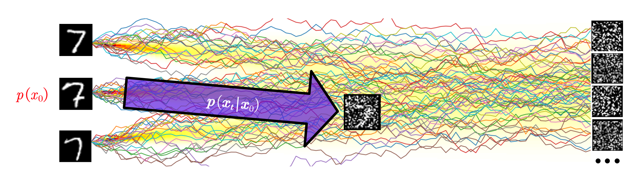
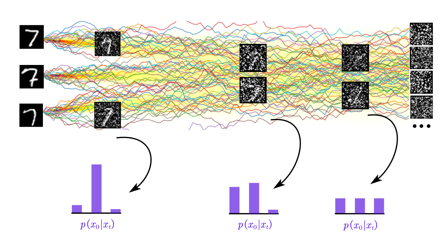
In this formula, the meaning behind the math is then straightforward, as shown in the figure above: During training, we randomly sample an image $x_0$ from the data distribution $p(x_0)$, and then add noise to form $x_t$ (or, mathematically, sampling from $p(x_t\mid x_0)$ to get $x_t$).

However, if we switch to the model’s perspective, then things are reversed.

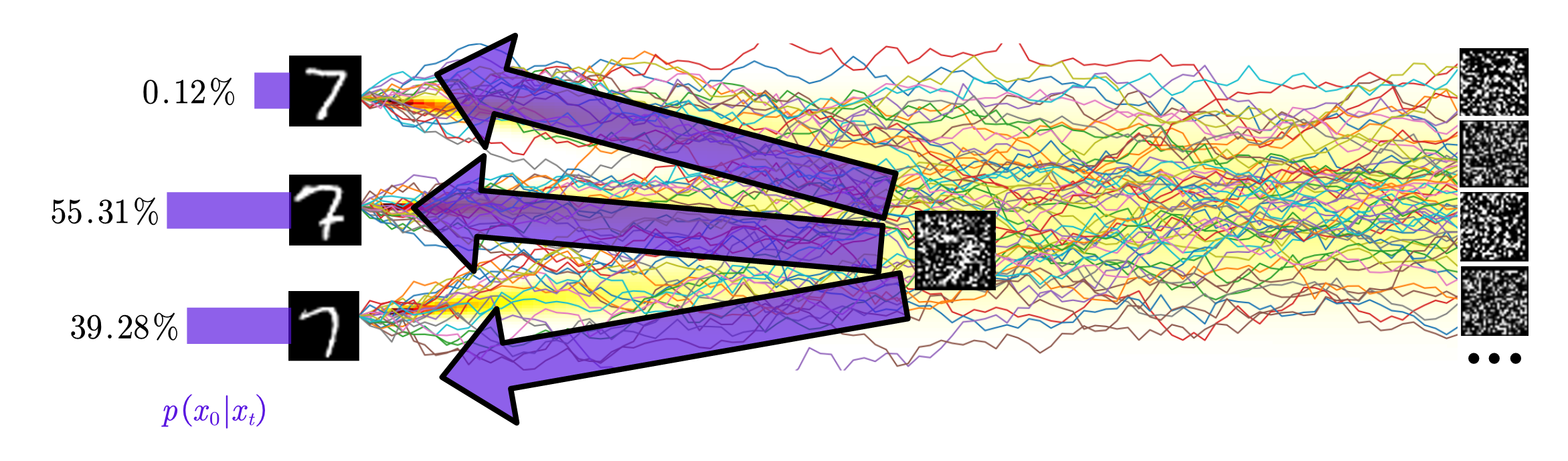
As the figure shows⁴, if we fix the input $x_t$ that the model is trained at, then the $x_0$ it received throughout the training course forms a distribution. This is just the posterior distribution $p(x_0\mid x_t)$:

\[p(x_0\mid x_t) = \frac{p(x_t\mid x_0)p(x_0)}{p(x_t)}.\]

We have finally reached our conclusion: the neural network tries to learn the posterior average among all clean images, conditioned on the input noisy image. In some sense, this is also why the task can be well-learned by the model: the task is strongly related to the traditional image restoration tasks, which have been well-studied in the deep learning community in the past.

Diving Into the Posterior Distribution

The posterior averaging formulation we discussed above is actually quite general. Not only that most of the diffusion models with various schedules (e.g. DDPM¹, iDDPM⁵, etc.) can be formulated as this, but the emerging flow matching models⁶, or 1-rectified flow⁷, are also special cases of this formulation.

It turns out that the posterior distribution $p(x_0\mid x_t)$ can be quite interesting, and its shape differs significantly at different timesteps. We can roughly divide the timesteps into three categories: small $t$, large $t$, and intermediate $t$, corresponding to the three “faces” of our denoising diffusion model.

1. Small $t$ : Denoising Stage

When $t$ is small, $x_t$ retains most of the original data, with only minor noise added. Thus, it is natural to expect that $p(x_0\mid x_t)$ is sharply peaked.

Formally, we can state this using the Bayes formula we wrote above:

\[p(x_0\mid x_t) \propto p(x_t\mid x_0)p(x_0)\]

Although theoretically, we should treat $x_0$ as chosen from the “data distribution” $p(x_0)$, in practice, what we only have is the 50,000 data points. Thus, we shall write $p(x_0)$ as a mixture of Dirac delta distributions:

\[p(x_0) = \frac{1}{N}\sum_{x_i\in \text{MNIST}} \delta(x_0 - x_i),\qquad N=50000.\]

With some calculations², we can calculate the distribution $p(x_t\mid x_0)$:

\[p(x_t\mid x_0) = \mathcal{N}(x_t; c_t x_0, d_t^2\mathbf{I}),\]

where $c_t$ and $d_t$ are also some human-readable functions of $t$. Combining them yields

\[p(x_0=x_i\mid x_t) = \text{Softmax}\left(\left\{-\frac{\|x_t-c_t x_j\|^2}{2d_t^2}\mid j=1,2,\cdots,N\right\}\right)_i\]

Moreover, for most of the designs, if we set $t=0$, then $c_t=1$ and $d_t=0$, in order to make $p(x_t\mid x_0)$ consistent. Thus, we can see that as $t\to 0$, the distribution $p(x_0\mid x_t)$ will be a Dirac delta function centered around the nearest neighbor of $x_t$ in the dataset, verifying our intuition.

Thus, in such cases, we can interpret the model’s task as just predicting the clean image, as demonstrated in the figure below.

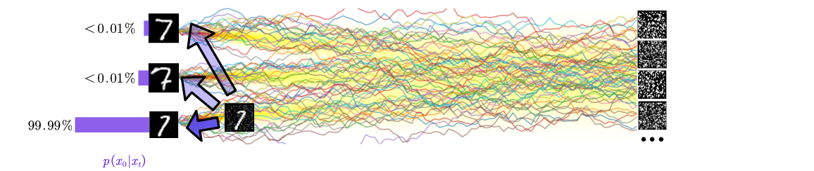
We can summarize the model’s task as a denoiser, distinguishing noise from the underlying signal.

2. Large $t$ : Statistics Learning

As $t$ approaches $T$, the noising process transforms the data distribution into $\mathcal{N}(0, I)$. Given an input $x_t$ sampled from the distribution, it can be expected that the model gains no information of which $x_0$ it is “come from”. Thus, the model should predict the mean of the dataset.

To be more precise, we can still use the formula above, and notice that as $t=1$, we should have $c_t=0$ and $d_t=1$, in which case the softmax scores

\[-\frac{\|x_t-c_t x_j\|^2}{2d_t^2} = -\frac{\|x_t\|^2}{2}\]

is no longer dependent on $j$. Thus, the distribution $p(x_0\mid x_t)$ will indeed be a uniform distribution over the dataset, as shown in the figure below.

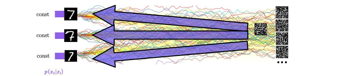
In this scenario, $p(x_0\mid x_t)$ approximates a uniform categorical distribution over $N$ discrete points, with equal probability assigned to all possible $x_0$. The model now focuses on learning the global statistics of the data, with the most obvious one being the mean of the dataset. The higher order statistics may also appear for $c_t\approx 0$ but $c_t> 0$, but we won’t dive into more details here.

3. Intermediate $t$ : Feature Learning

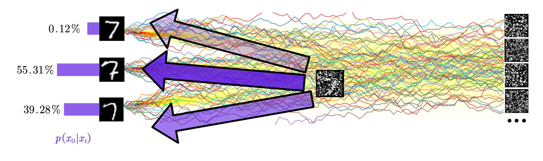
The most intriguing part actually lies in the middle part, where the posterior distribution is neither solely concentrated nor uniformly distributed. For example, it may place a reasonable amount (i.e. not too small or too large) probability weights on the many neighbors, as shown in the figure below.

However, this statement is very non-trivial, and maybe we should think more before taking it for granted. For example, just take a look at the three images below.

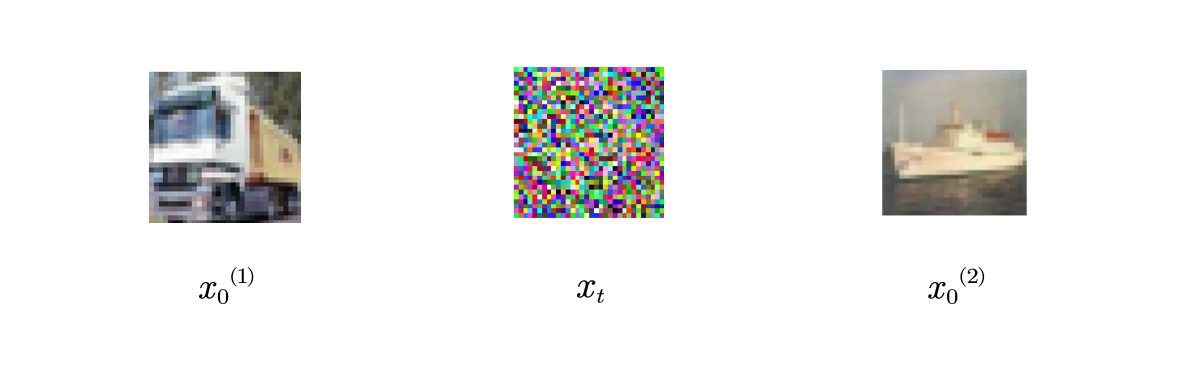
The middle image is an example input $x_t$ when $d_t\approx 0.8$ and $c_t\approx 0.2$, and the left and right are images chosen from the dataset. Now, if I don’t allow you to do any math calculation, just based on your built-in intuition of natural images, can you guess what’s the ratio of the two posterior probabilities

\[\frac{p(x_0^{(1)}\mid x_t)}{p(x_0^{(2)}\mid x_t)} ?\]

A common guess may be around 1. The mathematical truth, however, is astonishing: the ratio is on the order of $10^{4}$! This is not a joke, as we can immediately carry out a rule-of-thumb estimation:

• By the Gaussian Annulus Theorem, if you draw an sample from $p(x_t\mid x_0) = \mathcal{N}(x_t; 0.2 x_0, 0.8^2\mathbf{I})$, then it is likely that $|x_t-0.2x_0| \approx 0.8\sqrt{d}$, where $d$ is the dimension of the image;
• Let’s say, $d=32\times 32\times 3\approx 3000$. Then the typical $L_2$ distance between $0.2x_0$ and $x_t$ is on the order of 40.
• It turns out that the first image $0.2x_0^{(1)}$ is closer to the noise $x_t$, with a distance of around 44.25; $0.2x_0^{(2)}$ is little bit far away, with a distance of 44.40. This doesn’t sound like a big difference, but if you calculate the probability:

\[\frac{p(x_0^{(1)}\mid x_t)}{p(x_0^{(2)}\mid x_t)} = \frac{\exp(-\frac{44.25^2}{2\times 0.8^2})}{\exp(-\frac{44.40^2}{2\times 0.8^2})} \approx e^{10.4} \approx 3\times 10^{4}.\]

Of course, you may not be very comfortable with this hand-wavy calculation, but we also provided a notebook at here for you to verify this numerically.

So, why did you get this question wrong, even if you should be a human – a master of natural images? The answer is quite simple: you have generalize ability, which is indeed what makes you guess incorrectly in this case. The probability calculations above are on the CIFAR-10 dataset, which is just 50,000 images. However, what you “calculate” using your intuition is actually something like this:

\[\frac{p(x_0^{(1)}\mid x_t) + p(x_0^{(1)'}\mid x_t) + p(x_0^{(1)''}\mid x_t) + \cdots}{p(x_0^{(2)}\mid x_t) + p(x_0^{(2)'}\mid x_t) + p(x_0^{(2)''}\mid x_t) + \cdots} \approx 1.\]

Where $x_0^{(1)^\prime}, x_0^{(1)^{\prime \prime}}$ is all the images that you have seen or have imagined, that are semantically similar to the truck in the first image. For example, you will never notice if the truck is shifted by 1 pixel, or rotated by 1 degree, or even with something computers can’t even simulate, such as tilting only one wheel of the truck. However, despite all of these changes means nothing to you, they indeed changes the probability significantly. And finally there will be a term in the “$\cdots$” that contributes significantly to both the nominator and the denominator, which are definitely not in the dataset, but are what you “actually expect”.

Fortunately, however, the neural network is on your side: hopefully, it can capture what you have as a human, and do the exact thing as you did. In such a case, it will no longer be learning the sharply peaked distribution where the second closest neighbor has a probability factor of less than $10^{-27}$. Instead, it will try to build a “smooth” distribution, which is exactly what we discussed initially in this section.

Finally, let’s return to where we started: now we understand why the distribution is neither sharply peaked nor uniformly distributed at this intermediate stage. It also becomes clearer that this part is actually the most important for the model to have a good generalization ability. Instead of the stages we discussed previously, where the model learns something we can describe mathematically (such as the denoising task or learning statistics), the model is actually learning “features”, matching the “semantic parts” of the input $x_t$ with the possible “modes” of $x_0$ that it can imagine.

Summary

Let us recall the three faces of the diffusion model, separated (roughly) by the amplitude of the time step:

• Small $t$: Denoiser, predicting clean images from noisy inputs.
• Large $t$: Statistics learner, capturing global data statistics.
• Intermediate $t$: Feature learner, where generalization really happens, and the model learns the semantics and patterns.

With the three stages clearly explained (although the boundaries between them are indeed blurry), there also naturally emerges a question: Which part is the bottleneck?

Indeed, this question may lead to various answers, and it is hard to prove whether one answer is correct or not. However, we can state our own opinion here: The bottleneck actually lies in the intermediate stage. As we have mentioned, the intermediate stage is the stage that requires the model’s generalization ability the most, and it is also the stage where the model must learn some semantical meanings from, instead of memorizing the data. We are excited to see some cleverly designed experiments that can verify or disprove this hypothesis in the future.

Decoupling the Tasks

We have already seen the three faces of the diffusion models. However, one can notice that the three stages are actually not that closely related, and it might be not optimal for a single model to try to learn all of them together. Decoupling them is thus a natural idea to consider.

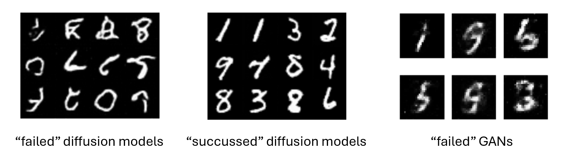
Decoupling the three tasks can indeed lead to efficiency. For example, we know that VAE models are fast one-step generators, but suffer from blurry images. In our language, they are quite good with the “feature learning” part, but it lacks a final “denoising” step. On the other hand, diffusion models are slow, but most of their steps are actually spent on the “feature learning” part. Also, if you have trained a diffusion model but failed to generate high-quality images, you will notice that its generations are very sharp (i.e. without noise or blurring parts), but only the shape is wrong. This is very different compared with other methods such as GANs (see the image below⁸), demonstrating the strength of diffusion models on the “denoising” part.

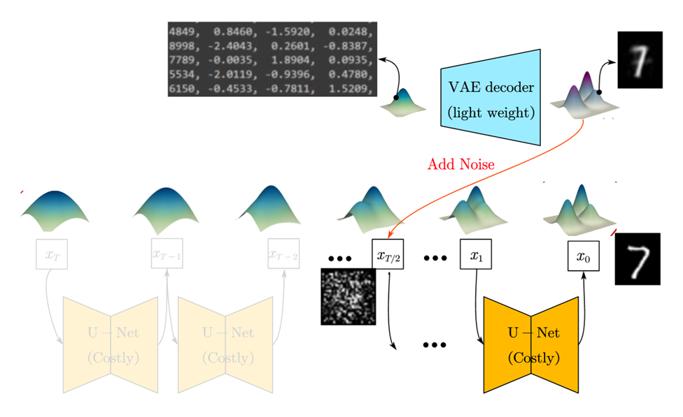
Our idea is thus combining the benefits of the two models. We use a very lightweight VAE decoder to generate blurry images. Then, we add noise to the VAE-generated images, and use a diffusion model to re-denoise it, to get a more high-quality image, as shown in the figure below⁹. Note that half of the diffusion steps are not needed, so we can achieve a 2x speed up.

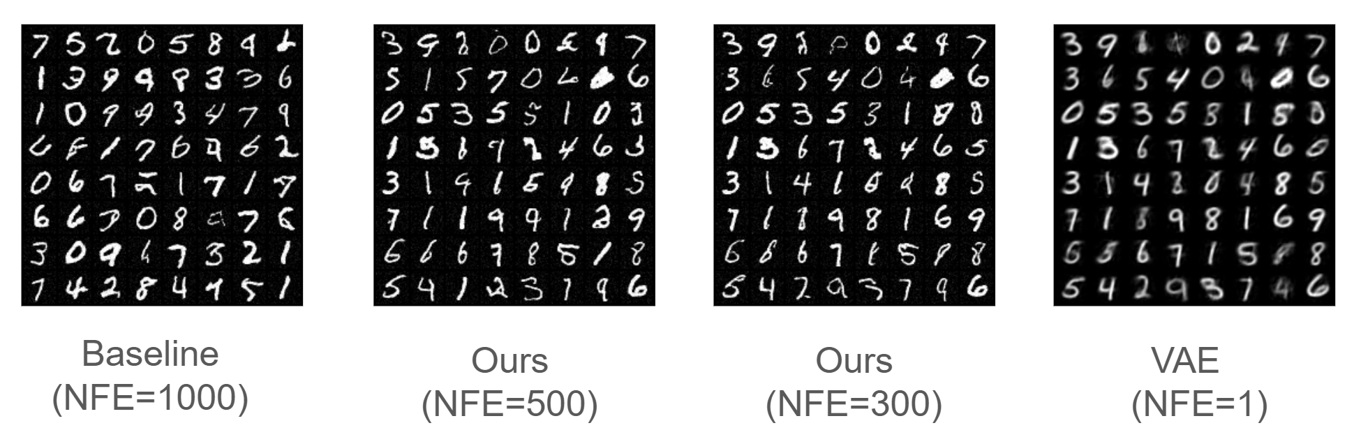
Based on our experiment results¹⁰ on the MNIST dataset, the method retains the sample quality reasonably, while achieving a 2x (or more) speed up compared with the original diffusion model, as shown in the figure below.

It’s worth noting that this experiment is just a simple demonstration of the idea of decoupling the tasks. We believe that the concept can be further extended and open the door to more efficient diffusion model pipelines in the future.

Conclusion

Diffusion models, since their birth in around 2015, have experienced rapid development and enormous improvements in the past ten years. Although their formulations or algorithms become increasingly complex with very fancy mathematics, we should always remember their essence, and what the model is actually learning. This is exactly what we hope to have clarified in this post using the three faces of the diffusion model.

We also sincerely hope that this post, along with the understanding of the three faces, can inspire more researchers to re-think the design of the diffusion models, and to further improve the efficiency and the quality of them in the future.

1. Ho, Jonathan, Ajay Jain, and Pieter Abbeel. “Denoising diffusion probabilistic models.” Advances in neural information processing systems 33 (2020): 6840-6851. ↩ ↩²

2. Weng, Lilian. (Jul 2021). What are diffusion models? Lil’Log. https://lilianweng.github.io/posts/2021-07-11-diffusion-models/. ↩ ↩²

3. He, Kaiming, et al. “Deep residual learning for image recognition.” Proceedings of the IEEE conference on computer vision and pattern recognition. 2016. ↩

4. Note: the numbers inside the figure are made up, same for the figures afterward. ↩

5. Nichol, Alexander Quinn, and Prafulla Dhariwal. “Improved denoising diffusion probabilistic models.” International conference on machine learning. PMLR, 2021. ↩

6. Lipman, Yaron, et al. “Flow matching for generative modeling.” arXiv preprint arXiv:2210.02747 (2022). ↩

7. Liu, Xingchao, Chengyue Gong, and Qiang Liu. “Flow straight and fast: Learning to generate and transfer data with rectified flow.” arXiv preprint arXiv:2209.03003 (2022). ↩

8. The image generated by GAN is taken from web: https://github.com/sssingh/mnist-digit-generation-gan/blob/master/assets/generated_images_epoch_50.png ↩

9. Image credit: https://mit-6s978.github.io/ ↩

10. See our code at https://github.com/Hope7Happiness/6s978_project ↩